

The stock market is a child with a stick…
The stock market is a child with a stick…
…and eventually, the stick breaks, and the kid cries until it finds a new one.

I want to start this article with a quote from Daniel Kahneman and Amos Tversky.
The predicted value is selected so that the standing of the case in the distribution of outcomes matches its standing in the distribution of impressions. [1]
That means that analysts and people generally tend to predict based on similarities or known events. An analyst who estimates a small business’s sales would use its database about similar companies and predict based on those numbers.
We often have singular information – a company that sells books – and a large number and distributed number of outcomes for similar cases. A good example is Amazon. In the beginning, analysts looked at Amazon as an online book store that ought to behave similarly to other bookstores in the brick & mortar world. So the predicted value was based on a known outcome.
The core idea of the paper [2] – Does the stock market overreact? – is that markets tend to overweight recent data and underweight the base rate.
John Maynard Keynes summarized the irrationality of markets nicely
Day-to-day fluctuations in the profits of existing investments, which are obviously of an ephemeral and non-significant character, tend to have an altogether excessive, and even an absurd, influence on the market. [3]
In other words, nothing about the fundamentals of a company changes, but the stock price can drop by 30% on a whim or negative comment in a newspaper.
The paper’s hypothesis is as follows – If stock prices systematically overshoot, then their reversal should be predictable from past return data, just by looking at the multiples that it is and has been trading at. This is the Overreaction Hypothesis.
We can split the hypothesis into two parts:
When the stock price moves extensively up/down, we’ll see a subsequent reversal of that movement in the other direction.
The more extreme the movement in either direction, the greater the subsequent reversal will be.
Interestingly enough, this is the basis for one of the valuation tools I frequently use – Fastgraphs.
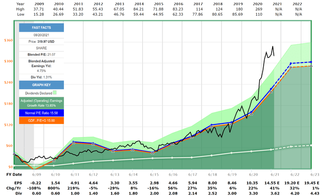
Source: Fastgraphs.com
On the Fastgraph, you see the price of the stock in black, the normal P/E ratio based on past calculated P/E ratios in blue, the orange line depicts an on valuation models calculated P/E ratio, the dark green area shows the earnings, and the light green area the dividend payout.
In Fastgraphs, it depends strongly over which time-horizon you look. While the stock in the picture above looks dramatically overpriced, it’s taking the great financial crisis into account, which depresses the multiple calculations strongly. If I reduce the time window, the multiple is recalculated with more up-to-date multiples, which results in a more realistic valuation.
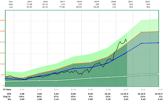
One of two things most commonly happens if the black graph deviates strongly from the orange or blue line.
A price correction back to the historical mean
Stagnation in price while the fundamentals catch up over time
You could ask, which one of these two things happens faster? I’d say it really depends on the market’s mood. If the general economy is doing ok, prices can stay elevated for quite some time until the fundamentals catch up. If the economy is shaky, one bad news is enough to lead to a price correction.
Test Procedure
To show the validity of the Overreaction Hypothesis, Thaler and Bondt built winner and loser portfolios with stocks that have at least 85 months of return data. The returns will be measured 16 times from 1930 until 1975, which means roughly every 3 years.
Excess return is measured through the formula: ujt = Rjt – Rmt. With ujt being the excess return of security ‘j‘ at the time ‘t,’ Rjt being the return of the security, and Rmt being the return of the market during the same time period.
Stocks will be added or removed based on either extreme capital gains or losses over a time period of up to 5 years. These stocks will be either called Winners (W) or Losers (L) solely based on past excess return rather than earnings.
December 1932 is the first time where cumulative excess returns are calculated for the stocks. This step is repeated 16 times from 1932 until 1977. The cumulative returns are ranked from low to high on each of these 16 portfolio formation dates, and the winner and loser portfolios are formed. Companies that land in the top 35 cumulative return segment are added to the winner portfolio, companies in the bottom 35 of cumulative returns are added to the loser portfolio.
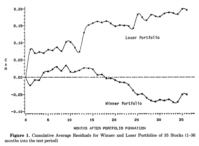
For each of these 16 non-overlapping three-year periods, the cumulative average residual returns (CAR) of all the securities in the portfolios are calculated for the next three years. During the next portfolio formation date, the winners and losers are reallocated based on their CARs.
The average CAR (ACAR) is calculated for the winner and loser portfolio during the whole period and each 3 year period.
The overreaction hypothesis dictates that ACAR(winner) < 0 and ACAR(losers) > 0. So that ACAR(loser) – ACAR(winner) > 0
Results
During the time period from 1930 to 1980, the loser portfolio outperformed the market on average by 19.6% after each of the 36 months after portfolio formation. The winner portfolio underperformed the market on average by 5%. This leads us to a difference in cumulative returns of
ACAR(loser) – ACAR(winner) = 24.6%
Further important findings:
The overreaction is asymmetric, meaning that the effect is smaller for the winners than for the losers.
Most excess returns in loser portfolios are realized in January
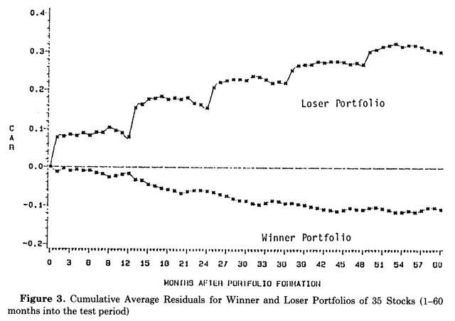
In agreement with Benjamin Graham’s claim – the overreaction phenomenon occurs during the second and third years.
The larger CARs during the formation period for winners and losers, the larger the reversals.
For each three-year period, the betas of the winner portfolios are on average 1.369 for the loser 1.026, which implies that the loser portfolio is also less risky than the winner portfolios.
We see a strong decline in the loser portfolio from October – December, which correlates strongly with the inclination of investors to tax-loss selling. The winner portfolio gains during these months and loses some in January.
Conclusion
Most people “overreact” to dramatic news events. In agreement with the overreaction hypothesis stated at the beginning of this article, a portfolio of “losers” outperformed a portfolio of “winners” by about 25% through the time period.
The limitations of this research are that we’re limited to stocks that have extensive data and exist throughout a long time period. This limits us somewhat to the largest companies within the stock market. High-growth stocks or ‘high-conviction’ stocks are not considered in this research.
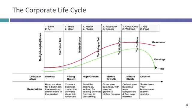
The time period over which this research was done was a slower pace environment. Companies usually go through cycles like this.
Source:
During the 20th century, this life cycle diagram was much longer than it is now. GE took ~100 years to move through this life cycle, while new-age companies like Yahoo only take ~20 years.
Many other questions pop up, like why is January the largest return month?
How does this strategy apply to high-growth stocks?
What about companies that are in their “End Game”?
What’s the influence of a companies fundamentals?
If following the overreaction hypothesis, I would make sure not to invest in companies that are at the end of their life but in a high-growth or mature growth state.
We can also add a macroeconomic perspective to the overreaction hypothesis and look for companies that are deeply yet irrationally depressed because of recent news. Like energy and transportation companies in 2020.
Overall, this is an exciting finding and worth looking into. This strategy is very contrarian as it implied investing in places that other investors avoid. It definitely requires investors to have control over their emotions when investing in losers instead of winners.
References
[1] D. Kahneman and A. Tversky – “Intuitive Prediction: Biases and Corrective Procedures”
[2] Werner F. M. De Bondt, Richard Thaler – “Does the Stock Market Overreact?”
[3] John Maynard Keynes – “The General Theory Of Employment, Interest, and Money,” pp 153-154